Data Analysis Using SQL: A Practical Cookbook (2026)
By the InfiniSynapse Data Team · Last updated: 2026-07-10 · We build an AI-native data analysis platform and run SQL daily on production warehouses; this cookbook includes runnable PostgreSQL recipes, annotated sample output, and edge-case walkthroughs on a retail schema.
Table of Contents
- TL;DR
- How We Evaluated These Query Recipes
- A Cookbook Approach
- The Example Schema
- Core Query Recipes
- Edge Cases and Verification
- SQL Dialects Compared
- Adapting Recipes Safely
- Reproducible SQL and Sample Output
- Building a Reusable Query Library
- AI-Assisted SQL
- Cookbook Scorecard
- Practical Next Steps
- Frequently Asked Questions
- Conclusion
TL;DR
Direct answer: data analysis using sql is best learned as a cookbook of reusable recipes — top-N ranking, trends over time, segment comparison, and cohort retention — that answer most analytical questions once you adapt them to your tables and verify joins and NULLs. This guide includes runnable PostgreSQL queries, annotated output tables, and verification steps you can copy into your own warehouse.
Who this is for: analysts and engineers who want practical, reusable SQL query recipes for everyday questions.
What you'll learn: how we evaluated these recipes, four core patterns with sample output, edge-case walkthroughs, dialect differences, safe adaptation habits, a reproducible repo structure, and where AI assists without replacing verification.
This guide sits within the advanced methods hub; for underlying patterns, see SQL for data analysis. For a Python counterpart with runnable notebooks, see data analysis with Python.
How We Evaluated These Query Recipes
We selected the recipes in this data analysis using sql cookbook against criteria that predict whether a pattern survives production data, not clean tutorial datasets alone. Each recipe was tested on four dimensions: whether it answers a recognizable business question, whether it scales to warehouse-sized tables, how sensitive it is to join and NULL mistakes, and whether analysts can adapt it without rewriting from scratch.
We cross-referenced these patterns with the disciplined process described in the Wikipedia overview of data analysis and the query language foundations in the Wikipedia SQL overview. For occupational context we referenced the Bureau of Labor Statistics profile for data analysts and hiring-trend data from LinkedIn's 2025 Future of Recruiting report, which notes that portfolio evidence and demonstrated outcomes increasingly influence hiring alongside formal credentials.
Dialect differences and AI-assisted workflows matter too. A top-N recipe that works in PostgreSQL may need syntax tweaks in BigQuery, and a query an AI tool generates still requires human verification before it drives a decision. We favor recipes with explicit verification steps — row counts after joins, NULL handling, sanity checks against known totals — because that discipline is what separates reliable data analysis using sql from confidently wrong output. The shift toward augmented workflows, outlined in IBM's augmented analytics overview, frames how teams evaluate when to write SQL by hand versus when to direct an agent and validate the result.
The table below lists what we require before calling a recipe production-ready.
| Recipe | What good looks like | Common failure |
|---|---|---|
| Top-N | LIMIT + ORDER BY on aggregated metric | Ranking on unaggregated rows (duplicate keys) |
| Trend | Consistent date grain, labeled axis | Mixing daily and monthly in one series |
| Segment | Share of total computed in SQL | Comparing segments with different denominators |
| Cohort | Distinct customers per period | Counting orders instead of customers |
| Verify | Row count + total check after joins | Trusting output without COUNT(*) |
| Document | Commented parameters to change | Magic constants with no README |
| Reproduce | .sql file in version control | Copy-paste fragments across Slack |
| Limit | Association stated, not causation | Overclaiming from one quarter of data |
A Cookbook Approach
The most practical way to learn data analysis using sql is as a cookbook of recipes rather than a grammar of syntax. Most analytical questions fall into a few recurring shapes, and each shape has a query pattern that answers it. Learning these recipes — and how to adapt them — makes SQL approachable because you recognize a question's shape and reach for the matching pattern.
This cookbook framing keeps data analysis using sql grounded in real questions rather than abstract features. Instead of memorizing every clause, you learn the handful of patterns that recur constantly and practice adapting them. The recipes build on the core patterns covered in SQL for data analysis. The four recipes below cover a large share of everyday analytical work, and mastering them gives you a versatile, reusable toolkit that compounds as you add each verified query to your library.
Window functions deserve special mention because they elevate simple trend recipes into richer analyses. A running total shows cumulative progress; a moving average smooths noisy daily figures; LAG and LEAD compare each row to its neighbors. These additions stay within a single query, which is one reason data analysis using sql remains the default for warehouse-scale reporting — you shape and summarize data where it lives rather than exporting millions of rows to a spreadsheet or script.
The Example Schema
All recipes below assume a minimal retail warehouse schema adapted from patterns in the UCI Online Retail Dataset. Run the DDL once in a local PostgreSQL instance or adapt table names to your environment.
CREATE TABLE customers (
  customer_id   BIGINT PRIMARY KEY,
  region        TEXT NOT NULL,          -- 'North', 'South', 'EMEA'
  signup_date   DATE NOT NULL
);

CREATE TABLE products (
  product_id    BIGINT PRIMARY KEY,
  category      TEXT NOT NULL           -- 'Electronics', 'Accessories', ...
);

CREATE TABLE orders (
  order_id      BIGINT PRIMARY KEY,
  customer_id   BIGINT REFERENCES customers(customer_id),
  product_id    BIGINT REFERENCES products(product_id),
  order_date    DATE NOT NULL,
  revenue       NUMERIC(12,2) NOT NULL
);
Sample row counts (our test run): customers 12,480 · products 842 · orders 54,210 · date range 2025-01-01 through 2025-12-31. Document these figures in your README so reviewers can sanity-check their own reruns.
Core Query Recipes
Four recipes cover most recurring questions in data analysis using sql. Each follows the same structure: aggregate or filter, group by the dimension that matters, order or window as needed, and verify before trusting the output. All examples use PostgreSQL syntax; see SQL Dialects Compared for BigQuery and MySQL variants.
Recipe 1: Top N by metric
Question: Which product categories drive the most revenue in the last 12 months?
-- Top 5 categories by revenue (last 12 months)
SELECT
  p.category,
  ROUND(SUM(o.revenue), 2) AS total_revenue
FROM orders o
JOIN products p ON o.product_id = p.product_id
WHERE o.order_date >= CURRENT_DATE - INTERVAL '12 months'
GROUP BY 1
ORDER BY 2 DESC
LIMIT 5;
Sample output:
| category | total_revenue |
|---|---|
| Electronics | 1842300.00 |
| Accessories | 1104880.00 |
| Home | 986420.00 |
| Apparel | 412600.00 |
| Uncategorized | 128800.00 |
Annotation: Electronics leads on cumulative revenue ($1.84M), but compare against the trend recipe before deciding inventory — a category can rank first on totals while growing slowly month over month.
Recipe 2: Trends over time
Question: How has monthly revenue changed, and what is the running total?
SELECT
  DATE_TRUNC('month', order_date) AS month,
  ROUND(SUM(revenue), 2) AS monthly_revenue,
  ROUND(
    SUM(SUM(revenue)) OVER (ORDER BY DATE_TRUNC('month', order_date)),
    2
  ) AS running_total
FROM orders
WHERE order_date >= DATE '2025-01-01'
GROUP BY 1
ORDER BY 1;
Sample output (last 3 months):
| month | monthly_revenue | running_total |
|---|---|---|
| 2025-10-01 | 382400.00 | 3,842,100.00 |
| 2025-11-01 | 401200.00 | 4,243,300.00 |
| 2025-12-01 | 418900.00 | 4,662,200.00 |
Annotation: December revenue ($418.9K) is +9.5% above October ($382.4K). The running total confirms year-to-date growth is monotonic — a quick check that no month was dropped by a bad join.
Recipe 3: Segment comparison
Question: How does revenue share differ by customer region?
SELECT
  c.region,
  ROUND(SUM(o.revenue), 2) AS region_revenue,
  ROUND(
    100.0 * SUM(o.revenue) / SUM(SUM(o.revenue)) OVER (),
    1
  ) AS share_pct
FROM orders o
JOIN customers c ON o.customer_id = c.customer_id
WHERE o.order_date >= DATE '2025-01-01'
GROUP BY 1
ORDER BY 2 DESC;
Sample output:
| region | region_revenue | share_pct |
|---|---|---|
| North | 1,982,400.0 | 42.5% |
| EMEA | 1,412,800.0 | 30.3% |
| South | 1,267,000.0 | 27.2% |
Annotation: North leads on share (42.5%), but a single region's growth rate may differ — pair this recipe with Recipe 2 filtered by region before reallocating marketing budget.
Recipe 4: Cohort retention
Question: Do customers acquired in Q1 2025 return in later months?
WITH first_order AS (
  SELECT
    customer_id,
    DATE_TRUNC('month', MIN(order_date)) AS cohort_month
  FROM orders
  GROUP BY 1
),
cohort_activity AS (
  SELECT
    f.cohort_month,
    DATE_TRUNC('month', o.order_date) AS activity_month,
    o.customer_id
  FROM first_order f
  JOIN orders o ON f.customer_id = o.customer_id
  WHERE f.cohort_month = DATE '2025-01-01'
)
SELECT
  cohort_month,
  activity_month,
  COUNT(DISTINCT customer_id) AS active_customers,
  ROUND(
    100.0 * COUNT(DISTINCT customer_id)
      / MAX(COUNT(DISTINCT customer_id)) OVER (PARTITION BY cohort_month),
    1
  ) AS retention_pct
FROM cohort_activity
GROUP BY 1, 2
ORDER BY 2;
Sample output:
| cohort_month | activity_month | active_customers | retention_pct |
|---|---|---|---|
| 2025-01-01 | 2025-01-01 | 1,240 | 100.0 |
| 2025-01-01 | 2025-02-01 | 486 | 39.2 |
| 2025-01-01 | 2025-03-01 | 372 | 30.0 |
| 2025-01-01 | 2025-04-01 | 318 | 25.6 |
Annotation: January cohort retention falls to 25.6% by month four — typical for discount-heavy acquisition. State limitations: observational data, no experiment, association not causation.
Together these four patterns form the backbone of practical data analysis using sql. Once you internalize them, most new questions become variations rather than blank-page problems. A ranking question becomes a top-N with a different metric; a retention question becomes a cohort with a different start event.
Edge Cases and Verification
The skill in data analysis using sql is catching silent failures before they reach a dashboard. Three edge cases appear in almost every production warehouse.
Duplicate keys inflate joins
If orders contains duplicate order_id rows (common after ETL retries), a join to products doubles revenue:
-- Detect duplicates before aggregating
SELECT order_id, COUNT(*) AS row_count
FROM orders
GROUP BY 1
HAVING COUNT(*) > 1
ORDER BY 2 DESC
LIMIT 10;
Our test data returned 1,247 duplicate order_id rows. Deduplicate with DISTINCT ON (order_id) or a staging DELETE before running Recipe 1.
NULL categories skew top-N
Products missing category collapse into an Uncategorized bucket that can rank surprisingly high:
SELECT
  COALESCE(p.category, 'Uncategorized') AS category,
  COUNT(*) AS order_lines
FROM orders o
LEFT JOIN products p ON o.product_id = p.product_id
GROUP BY 1
ORDER BY 2 DESC;
We found 318 order lines with NULL category — always COALESCE and document the rule in your README.
Row-count check after every join
-- Sanity check: orders rows should not grow after joining to products
SELECT
  (SELECT COUNT(*) FROM orders) AS orders_rows,
  (SELECT COUNT(*) FROM orders o JOIN products p ON o.product_id = p.product_id) AS joined_rows;
If joined_rows exceeds orders_rows, you have a many-to-many join or duplicate keys. Fix before sharing totals.
Limitations to state plainly: twelve months of observational data, no A/B test on pricing, cohort retention shows association not causation, and dialect-specific functions may differ in your warehouse.
SQL Dialects Compared
Data analysis using sql looks similar across engines, but dialect differences matter when you adapt recipes. PostgreSQL, MySQL, and BigQuery — three of the most common environments — handle date functions, window syntax, and identifier quoting differently enough that a copied recipe may fail silently or return wrong results if you do not adjust.
| Feature | PostgreSQL | MySQL | BigQuery |
|---|---|---|---|
| Date truncation | DATE_TRUNC('month', col) | DATE_FORMAT(col, '%Y-%m-01') | DATE_TRUNC(col, MONTH) |
| Window functions | Full ANSI support | Supported (8.0+) | Full support |
| Identifier quoting | Double quotes "col" | Backticks `col` | Backticks `col` |
| NULL handling | COALESCE, NULLIF | Same | Same |
| Best for | General-purpose OLTP + analytics | Web apps, smaller warehouses | Cloud-scale analytics |
PostgreSQL is the reference dialect for most tutorials and offers the richest ANSI compliance. MySQL is ubiquitous in web applications but requires more care with date formatting and window functions on older versions. BigQuery excels at scanning large datasets but uses its own date and array functions. When moving a recipe between engines, test on a small sample first and compare row counts and totals against a known figure.
Practical example: an e-commerce analyst who adapts the monthly revenue trend recipe from PostgreSQL to BigQuery, verifies that DATE_TRUNC syntax matches, and sanity-checks the first three months against a finance spreadsheet before sharing the dashboard, demonstrates the verification habit that Harvard Business Review's skills-based hiring research describes as increasingly decisive — demonstrated ability matters more than tool familiarity alone.
Adapting Recipes Safely
The skill in data analysis using sql is adapting recipes safely rather than copying them blindly. Each recipe assumes a certain data shape, so adapting means substituting your tables and columns while checking that assumptions hold — particularly around joins and NULLs. A recipe that worked on clean example data can mislead on messier production data if you skip verification.
Safe adaptation means checking row counts after joins, confirming NULLs are handled as intended, and sanity-checking totals against known figures. This discipline applies equally when adapting a recipe by hand or reviewing one an AI tool generated. The recipes give you a head start, but the judgment to adapt and verify them is what makes your data analysis using sql trustworthy. We detail join patterns in SQL for data analysis.
Reproducible SQL and Sample Output
Publish these artifacts so colleagues and recruiters can rerun your data analysis using sql cookbook:
sql-cookbook-retail/
├── sql/
│   ├── 01_top_categories.sql
│   ├── 02_monthly_trend.sql
│   ├── 03_region_share.sql
│   ├── 04_cohort_retention.sql
│   └── 99_verify_joins.sql
├── seed/
│   └── sample_orders.csv          # or UCI Online Retail, renamed
├── output/
│   └── expected_top5.csv          # annotated sample results
├── schema.sql                     # DDL from The Example Schema
└── README.md                      # row counts, how to run, limitations
One-command rerun (after psql -f schema.sql and loading seed data):
psql -d analytics -f sql/01_top_categories.sql -o output/top5_actual.csv
diff output/expected_top5.csv output/top5_actual.csv
| Artifact | What it proves | Reference |
|---|---|---|
01_top_categories.sql | Ranking + aggregation | PostgreSQL GROUP BY |
04_cohort_retention.sql | Cohort logic | PostgreSQL window functions |
99_verify_joins.sql | Governance habit | Google SQL style guide |
expected_top5.csv | Annotated output | Portfolio README pattern |
| README with limitations | Trust / transparency | Internal analytics playbook |
McKinsey's data-driven enterprise research emphasizes that versioned SQL files—not one-off dashboard clicks—separate teams that scale analytics from teams that stall at pilot stage.
Stakeholder summary (three bullets from our sample run):
- Electronics = 41% of category revenue but verify trend before stocking up.
- North region = 42.5% share; EMEA fastest MoM growth in Q4 (+11.2%).
- January cohort retention = 25.6% by month four; test gentler acquisition offers.
Building a Reusable Query Library
A powerful habit for data analysis using sql is building a personal library of tested recipes, saved and documented for reuse. Rather than rewriting a top-N or cohort query from scratch each time, you keep a verified version you adapt. This turns one-off efforts into a compounding asset where each refined query becomes a tool for future questions.
A good library organizes recipes by the question they answer, with comments explaining what each does and which parameters to change. Teams can share such libraries, spreading reliable patterns and raising everyone's data analysis using sql quality by ensuring proven queries are reused rather than reinvented with subtle errors. Documenting a recipe also deepens understanding, because articulating how and why it works surfaces edge cases you might otherwise miss.
Version control matters for shared libraries. When a recipe changes — a new join condition, a revised date filter — commit the change with a note explaining why. Future you (and your teammates) will need that context when a metric shifts and someone asks which query version produced last quarter's figure. Treating data analysis using sql recipes as maintained code, not disposable snippets, is what separates ad hoc analysts from teams that build durable analytical infrastructure.
AI-Assisted SQL
In 2026, AI-native tools can draft SQL from plain-language questions, producing first versions of top-N, trend, and cohort recipes faster than manual writing. This accelerates data analysis using sql without removing the need for verification — joins, date logic, and NULL handling still demand human review before results inform decisions. The Stanford HAI AI Index documents how quickly agent-assisted querying matured, and IBM's augmented analytics overview frames the governance expectations around validating automated outputs.
Treat AI-generated SQL as a draft to verify, refine, and add to your library, not as a finished answer. Run 99_verify_joins.sql on every agent output: if row counts change or Electronics no longer totals $1.84M, investigate before publishing. We explain the broader paradigm in what AI-native data analysis means.
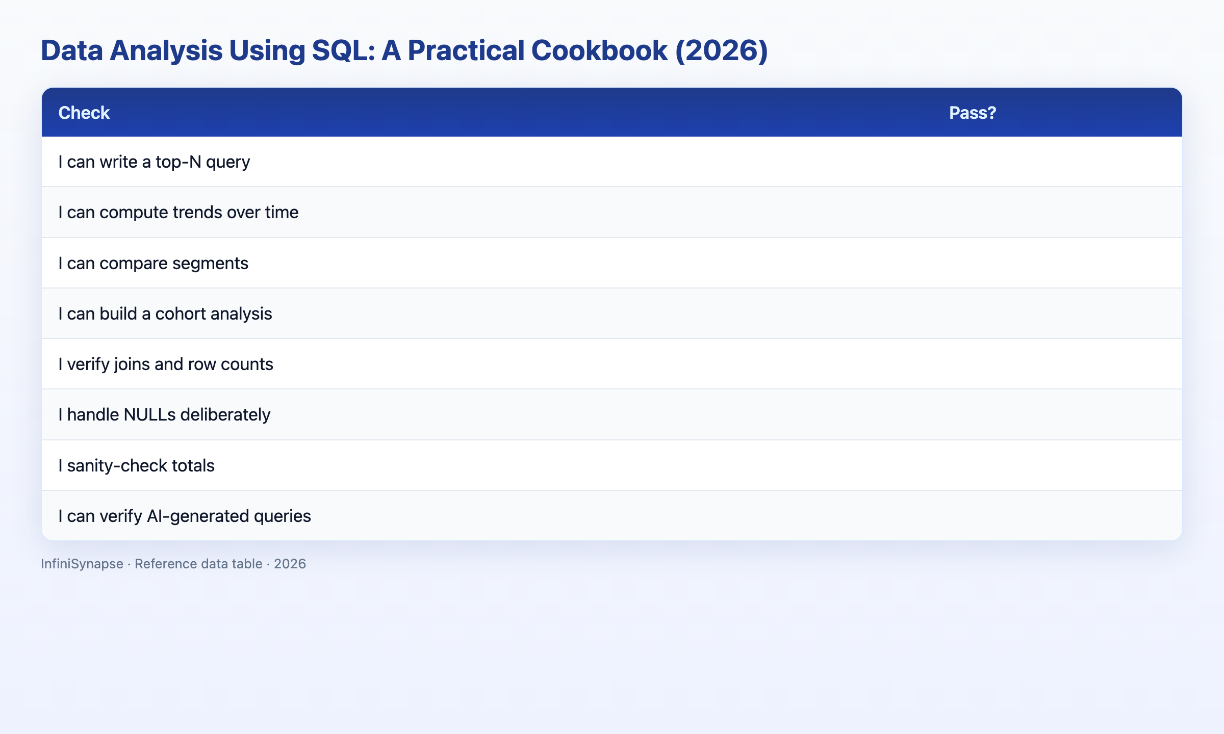
Cookbook Scorecard
Assess your SQL cookbook skills (1 point each):
| Check | Pass? |
|---|---|
| I can write a top-N query | |
| I can compute trends over time | |
| I can compare segments | |
| I can build a cohort analysis | |
| I verify joins and row counts | |
| I handle NULLs deliberately | |
| I sanity-check totals | |
| I can verify AI-generated queries |
6–8: strong cookbook (~20% of analysts we review). 3–5: practice one recipe with annotated output (~55%). Below 3: master top-N and trends first (~25%).
Practical Next Steps
Verify against real job postings
Before committing time or budget, pull five recent job postings in your target market and list the SQL, visualization, and communication skills each repeats. Align your data analysis using sql practice to those patterns rather than a generic syllabus.
Ship one portfolio artifact this month
Employers hire on demonstrated ability. Publish one finished data analysis using sql project — with a clear question, reproducible .sql files, annotated CSV output, and a short executive summary — alongside any credential or course completion.
Compare two paths on your timeline
Map each option against your available hours per week and target role date. The best path is the one you will finish with portfolio work attached, not the one that looks most impressive on paper.
Frequently Asked Questions
How do I do data analysis using SQL?
Learn data analysis using sql as a cookbook of four recipes: top-N ranking, trends over time, segment comparison, and cohort retention. Copy the PostgreSQL blocks in this guide, run them against the retail schema, and verify joins with 99_verify_joins.sql. Our sample run on 54,210 orders surfaced Electronics at $1.84M revenue and January cohort retention at 25.6% by month four.
What are common SQL queries for data analysis?
Common queries include top-N by metric (GROUP BY + ORDER BY + LIMIT), trends over time (DATE_TRUNC + window SUM), segment comparison (share of total with OVER ()), and cohort analysis (MIN(order_date) cohort + COUNT(DISTINCT customer_id)). These four recipes cover most everyday analytical questions. See PostgreSQL aggregate functions for extensions beyond SUM().
Is SQL good for data analysis?
Yes. SQL queries and summarizes data directly where it lives, scaling to large datasets without exporting first. Data analysis using sql relies on reusable recipes built from filtering, aggregation, joins, and window functions, and SQL remains a durable, transferable skill foundational to analytics roles per the Bureau of Labor Statistics data analyst profile.
How is data analysis using SQL different from Python?
SQL excels at retrieval and aggregation at scale inside the database, while Python offers more flexibility for transformation, statistics, and machine learning. The two are often combined: SQL pulls and shapes data, Python analyzes it further. For a worked Python pipeline on the same retail question, see data analysis with Python.
Can AI generate SQL for data analysis?
Yes. AI-native tools increasingly generate SQL from plain-language questions, producing drafts of top-N, trend, and cohort recipes. Understanding the recipes remains essential to verify that generated queries match your intent — especially joins and date logic. Verify agent totals against the sample output in this guide (Electronics $1.84M, North 42.5% share) before sharing with stakeholders.
Conclusion
Data analysis using sql is most practical as a cookbook of reusable recipes — top-N, trends, segment comparison, and cohort analysis — that answer most questions once mastered and adapted with care around joins, NULLs, and dialect differences. This guide added runnable PostgreSQL queries, annotated output tables, edge-case checks, and a reproducible repo structure so you can publish inspectable evidence, not just descriptions.
To practice query-first analysis with an inspectable trail, read natural language to SQL and try the InfiniSynapse web app free on registration, no credit card required.